1. Research background
Aircraft development programmes use aerodynamic databases built from wind-tunnel tests and CFD for design and performance assessment. Surrogate models trained on these existing data offer a way to provide rapid aerodynamic feedback during early design.
Deploying an AI model in an engineering organisation, however, involves more than predictive accuracy. Secure networks restrict file transfer and data sharing between machines, while the engineers who train a model and the designers who use its results work in different roles and environments. Training engineers have access to wind-tunnel and CFD data and GPU servers. Designers need rapid feedback on an ordinary workstation without having to operate a CFD solver or maintain an AI development environment.
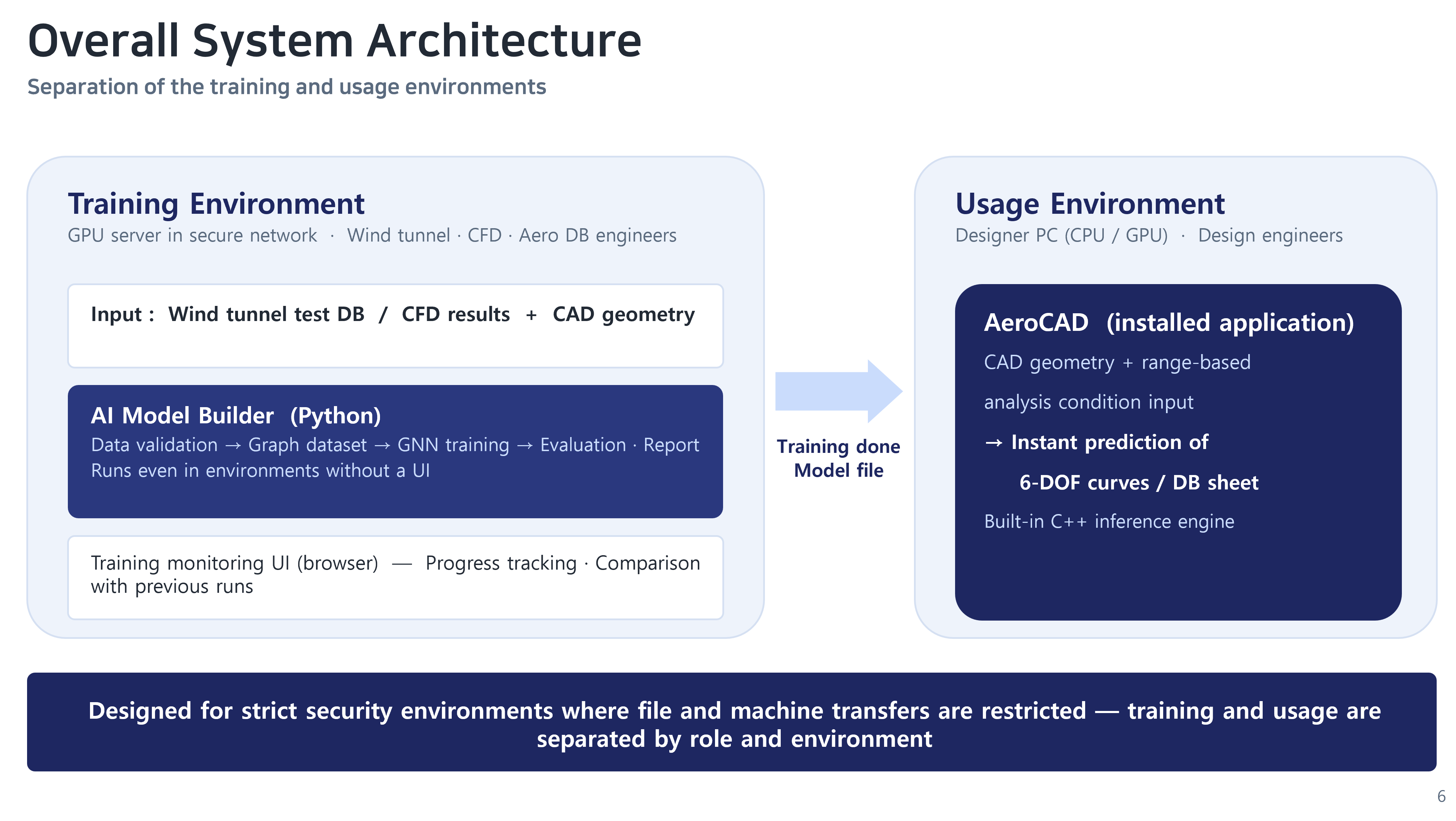
This study addresses those operating constraints with a GNN (Graph Neural Network) aerodynamic prediction system that separates the training environment from the user environment. The target outputs are the six force and moment coefficients of aircraft and helicopter bodies. The system consists of AI Model Builder for training and AeroCAD for desktop inference.
2. Separating model training from use
AI Model Builder: model production
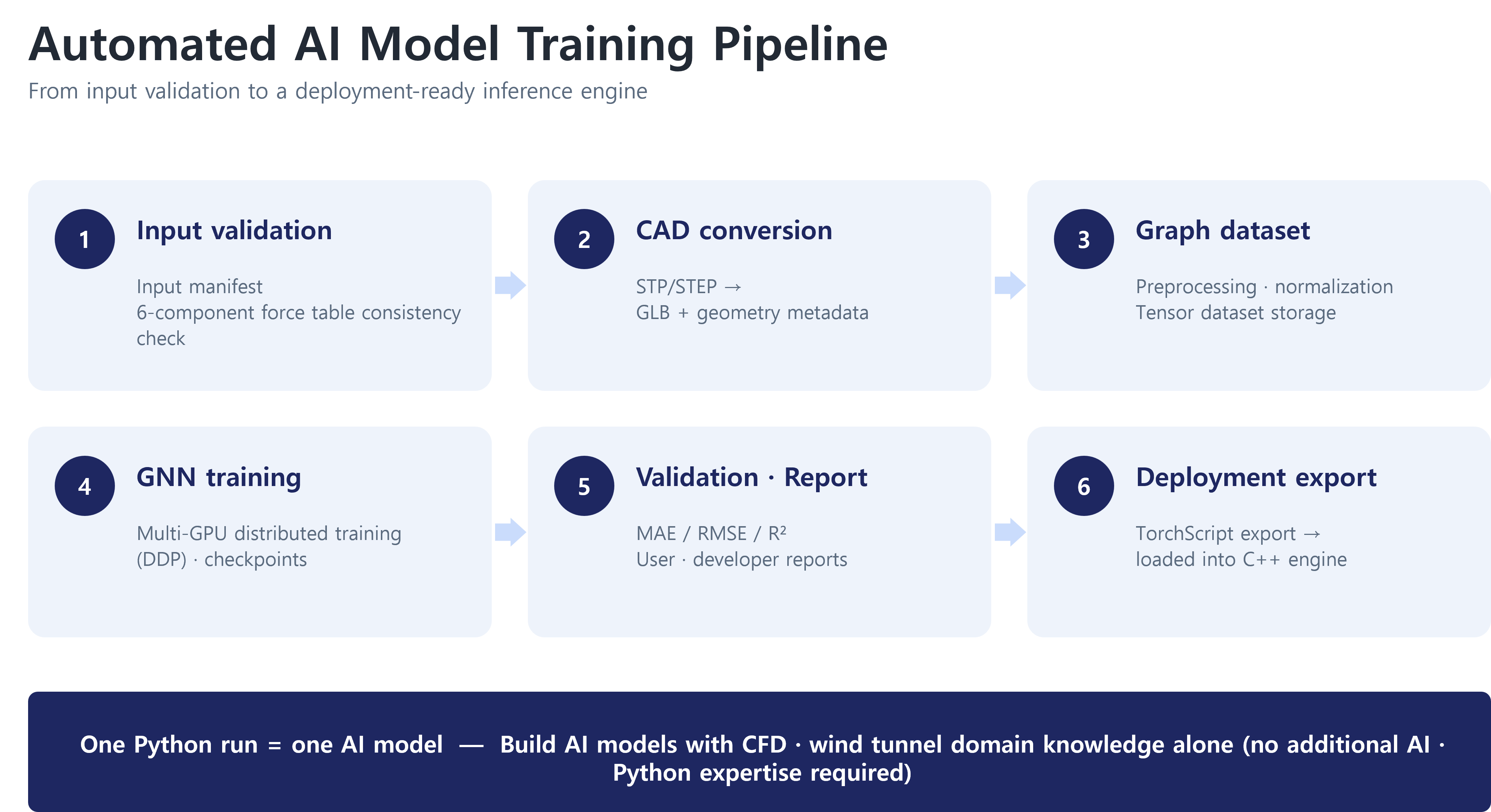
AI Model Builder accepts wind-tunnel or CFD results together with CAD geometry and automates the following stages:
- Validation of the input manifest and six-component coefficient tables
- Conversion of CAD geometry into a surface mesh
- Construction of the graph dataset
- Multi-GPU GNN training
- Evaluation and generation of user and developer reports
- Conversion of the trained model for deployment
The training engineer defines the physical meaning and application range of the data and arranges the dataset according to the input specification. The pipeline handles repetitive preprocessing, training, evaluation and deployment-package generation. The resulting model is transferred to the user environment with information describing its intended geometry and operating range.
AeroCAD: desktop inference
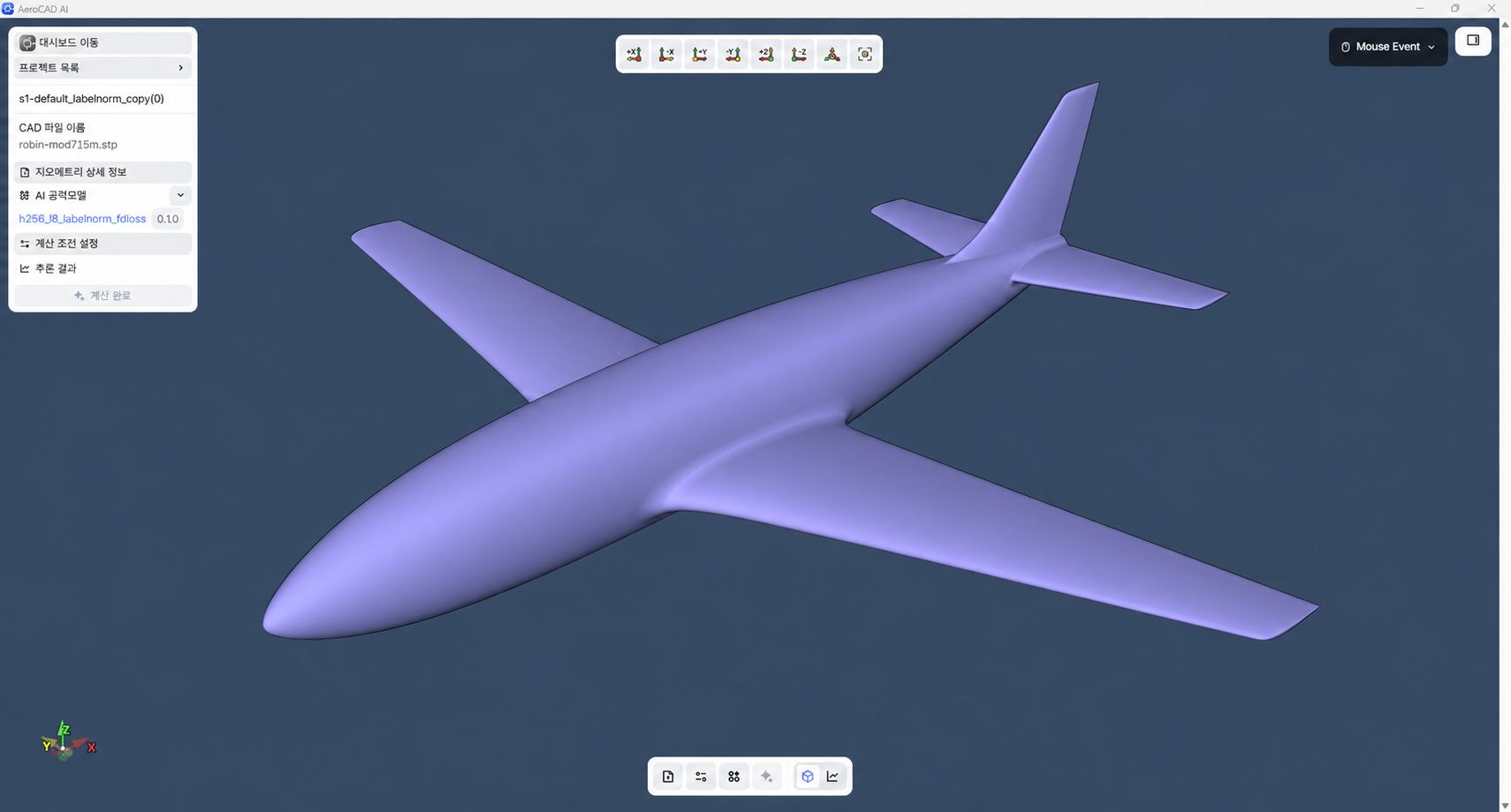
AeroCAD is an installed aerodynamic prediction application for designers. The user loads CAD geometry, enters ranges of Mach number, angle of attack (AoA) and sideslip angle (AoS), and selects a trained model appropriate for the case. AeroCAD evaluates the complete condition sweep and produces curves and database sheets for CFx, CFy, CFz, CMx, CMy and CMz.
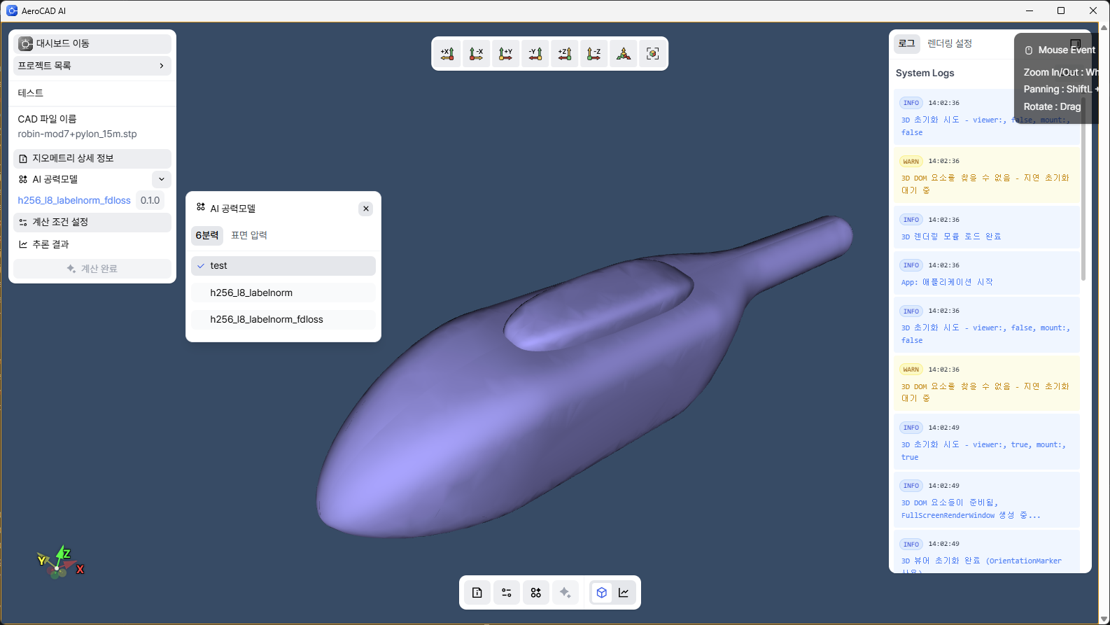
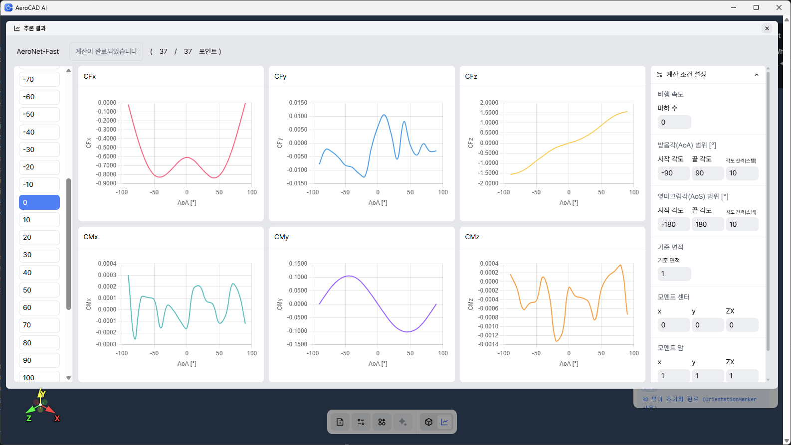
The inference engine is implemented in C++ and does not require a separate Python environment. It supports Windows and Linux and can run on either a CPU or GPU. Predictions, including tensor construction, are returned on a seconds-per-case timescale suitable for iterative design review.
3. Why represent the surface mesh as a graph?
Geometry can be supplied to a neural network through design parameters, fixed grids or images, or graph representations.
- Design-parameter representations are compact, but they cannot directly describe geometry outside a predefined parameterisation and must be rebuilt for each geometry family.
- Fixed-grid or image representations work naturally with architectures such as CNNs, but arbitrary topology and changes in mesh resolution are difficult to handle in a common input format.
- Graph representations retain the connectivity of an unstructured surface mesh and allow one model to process geometries with different node counts and connectivity.
The problem in this study is graph-level regression of integrated aerodynamic quantities. It predicts six-component coefficients from the surface graph and flight conditions; it does not predict the complete flow field.
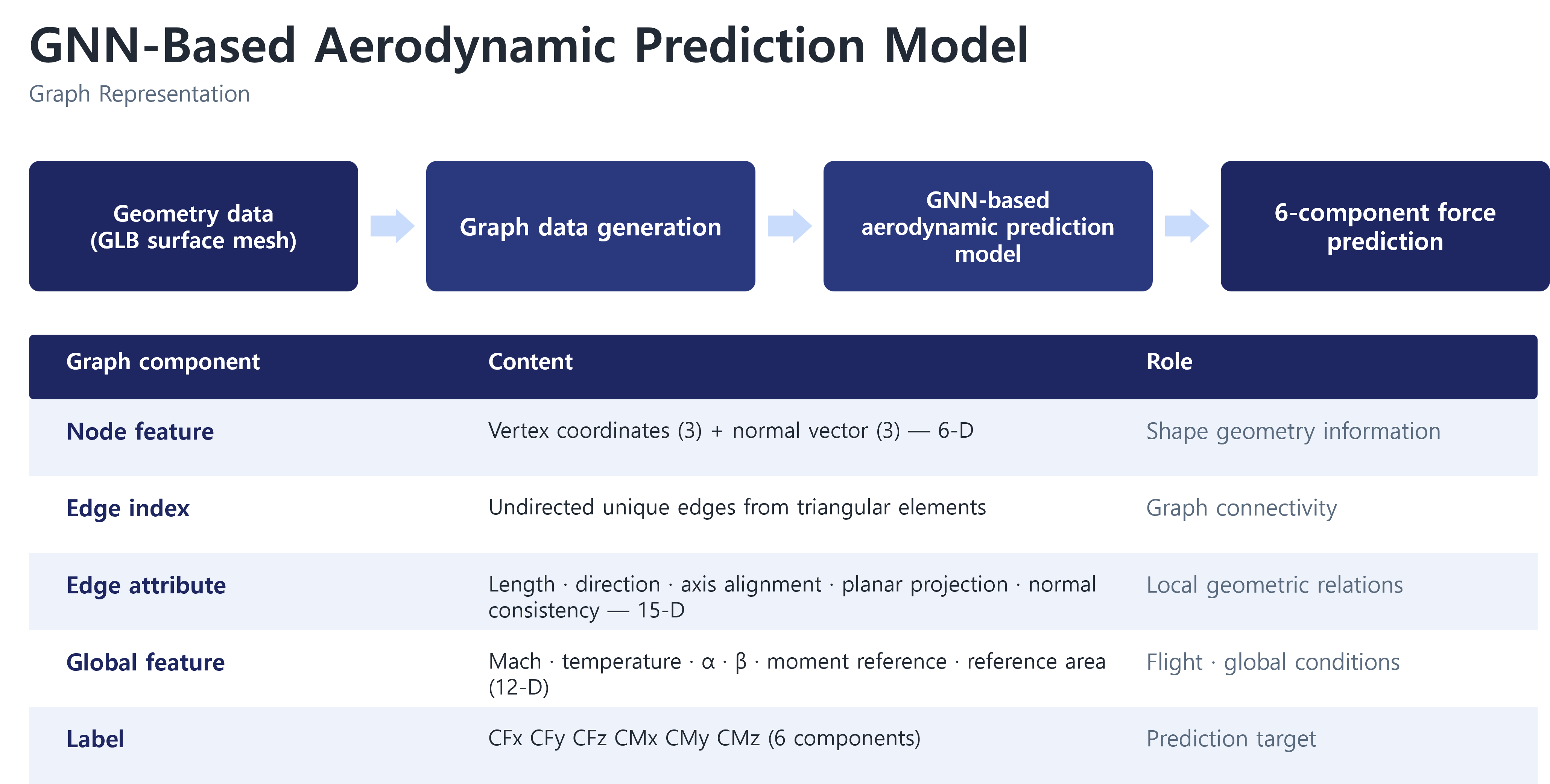
The graph input is constructed as follows.
| Component | Dimensions | Description |
|---|---|---|
| Node features | 6 | Three vertex coordinates and three components of the surface normal |
| Edge index | — | Unique undirected edges extracted from triangular surface elements |
| Edge attributes | 15 | Local geometric relations including length, direction, axis alignment, planar projection and normal consistency |
| Global features | 12 | Mach number, temperature, AoA, AoS, moment reference and reference area |
| Output labels | 6 | Three force coefficients and three moment coefficients |
4. GNN model and automated training
The input graph passes through a stack of message-passing layers that use the edge attributes. Global mean pooling then produces a graph-level geometry embedding, which is concatenated with the global flight-condition features. Fully connected output layers regress the six aerodynamic coefficients.
Separating training and deployment requires numerically consistent preprocessing in both environments. Node coordinates are centred and scaled by the bounding-box diagonal, while edge and global features use fixed transformations defined for each component. These transformations do not depend on dataset statistics, allowing the Python training pipeline and C++ inference engine to reproduce the same preprocessing. The six output coefficients are trained directly in their original scale without label normalisation.
The application study used 14 geometry variants derived from the ROBIN body. Combining geometry, Mach number, angle of attack and sideslip produced 19,166 samples. The training, validation and test sets were divided in an 8:1:1 ratio.
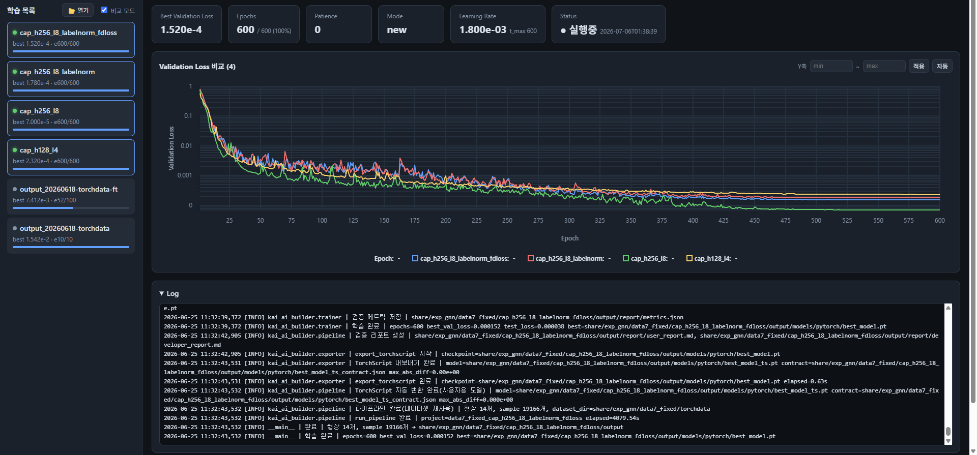
- Hidden dimension: 256
- Message-passing layers: 8
- Loss and optimiser: MSELoss and AdamW
- Training: multi-GPU distributed training with early stopping
- Convergence: stable convergence observed by 600 epochs
The monitoring interface reads training artefacts without modifying the training process. It displays the loss history, best epoch, learning rate and live logs, and compares multiple runs produced with different model configurations.
5. C++ inference and deployment
The training pipeline converts the final model to TorchScript. AeroCAD’s embedded C++ inference engine loads this model, converts the GLB geometry and operating conditions into tensors using the same preprocessing as the training pipeline, and evaluates the requested condition sweep.
This arrangement avoids maintaining Python and training-framework versions on every designer workstation. Data preparation and model production remain on the training server, while the user environment receives only the functions needed to inspect geometry, enter conditions, run inference and review the results. It also provides a clear separation of responsibility where movement between machines is restricted.
6. Validation on unseen geometries
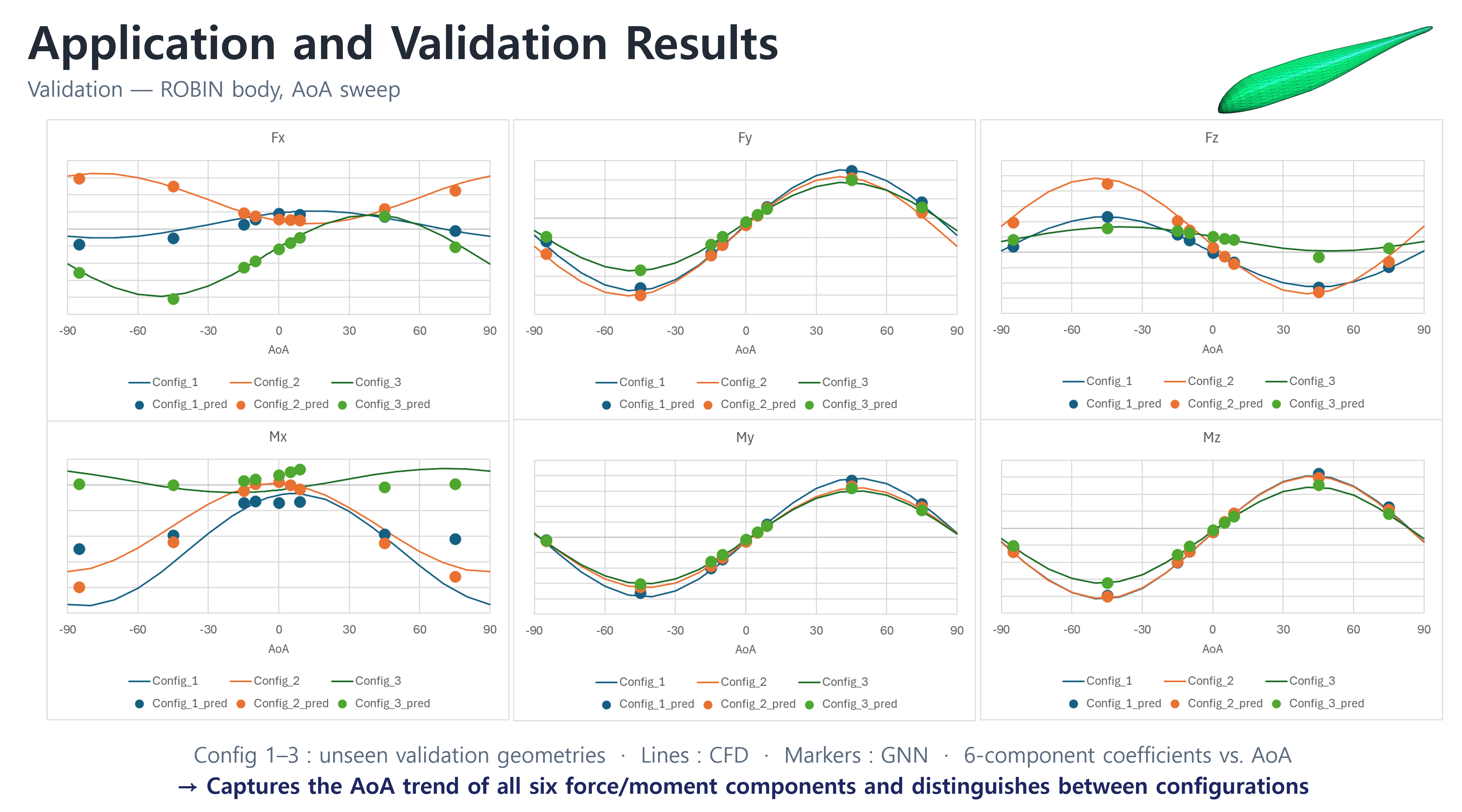
The model was evaluated on three ROBIN-derived configurations that were not included in training. Six-component predictions over an angle-of-attack sweep were compared with CFD results. Across the six outputs, the GNN followed the variation with angle of attack and distinguished the aerodynamic differences between the three configurations. Components whose absolute values were close to zero, particularly CFx and CMx, showed comparatively greater scatter.
Mesh-resolution robustness was examined separately. The same unseen geometry was remeshed at sizes ranging from approximately 50,000 to 700,000. Although only one reference mesh resolution was used in training, the predicted coefficients remained nearly unchanged when the mesh size varied by more than an order of magnitude.
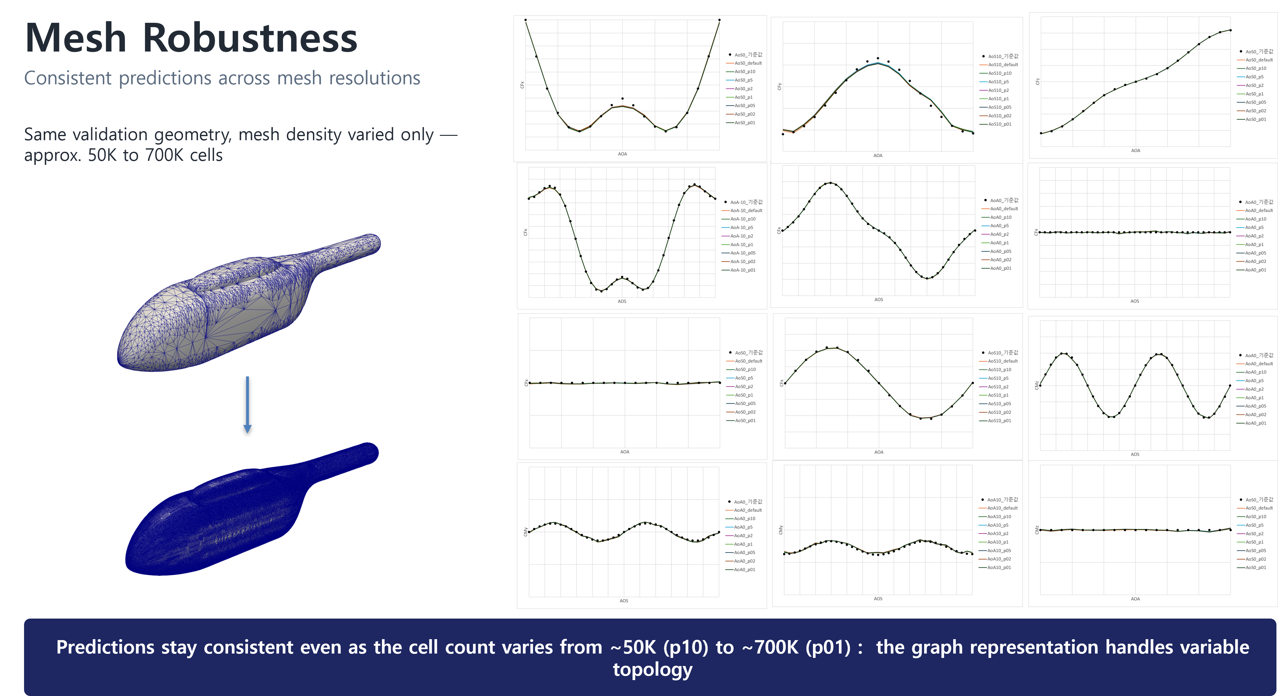
Within the geometry and mesh range tested here, this result demonstrates consistent handling of variable graph topology and mesh resolution. It does not establish generalisation across all aircraft geometries; broader application ranges require additional training data and validation.
7. Conclusion
This study developed a GNN model and operating system that reuse existing wind-tunnel and CFD data to predict aircraft six-component aerodynamic coefficients. AI Model Builder automates data validation, training, evaluation and deployment, while AeroCAD provides curves and database sheets from geometry and flight conditions on a designer’s workstation.
For unseen configurations, the model distinguished geometry-dependent behaviour and followed the coefficient trends over angle of attack. It also produced consistent predictions on surface meshes ranging in size from approximately 50,000 to 700,000. The intended role is not final performance assessment in place of high-fidelity CFD, but rapid trend evaluation during design and selection of geometries and conditions that warrant detailed analysis.
Future work will expand the geometry set to evaluate generalisation to three-dimensional fixed-wing aircraft and extend the model from integrated coefficients to surface pressure and skin-friction distributions.