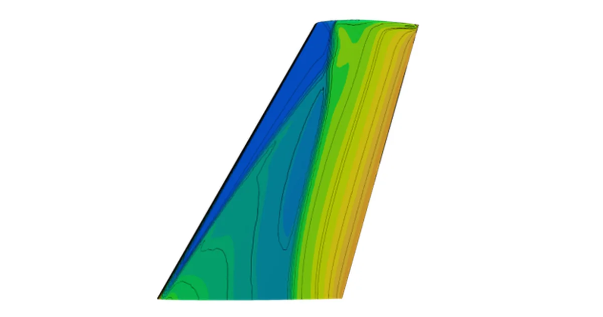
1. Overview
The ONERA M6 wing is well known in aircraft aerodynamics. Its combination of a simple geometry with a genuinely complex transonic flow makes it an ideal benchmark, and it is widely used to validate CFD codes for external flow. In this article we run a CFD analysis of that model on Flow360, a natively GPU-based solver.
More about Flexcompute Flow360, a next-generation CFD solver
2. Modelling and meshing
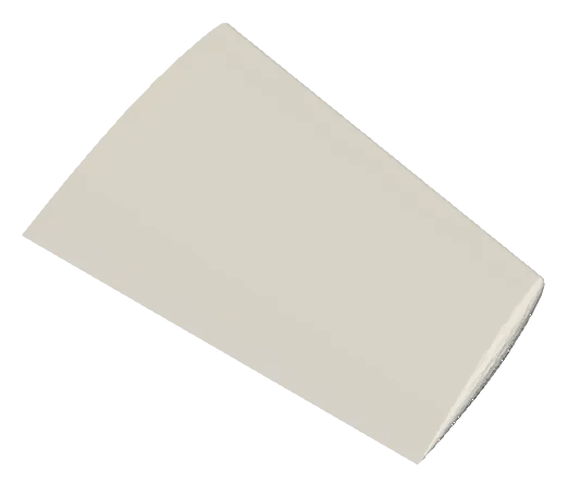
Detailed information on the ONERA M6 wing is available on the NASA website. This analysis uses a model normalised so that the wing root chord is 1 m, which gives the following geometric parameters.
- Mean aerodynamic chord (MAC) = 0.80167 m
- Semi-span = 1.47602 m
- Reference area = 1.15315 m^2
2.1 Domain
From this geometry we built the hemispherical domain commonly used for external flow analysis. Since this is a single-point case with no variation in angle of attack, a hemisphere is sufficient.
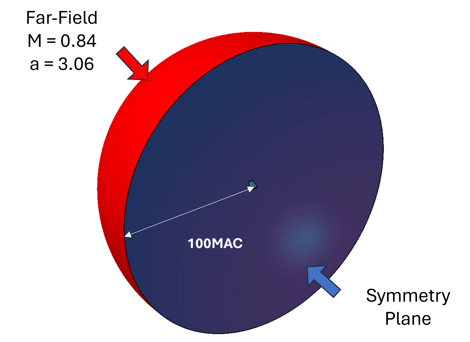
2.2 Meshes
Three meshes were built to examine grid dependence. Production work calls for a more thorough mesh study to get the most out of the available compute, but here the cell count was varied simply by adjusting the number of viscous layers and the near-field cell size.
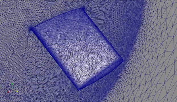
| Coarse | Medium | Fine | |
|---|---|---|---|
| Nodes | 1,728k | 3,856k | 4,948k |
| Cells | 7,246k | 20,807k | 25,473k |
3. Analysis conditions
3.1 Flow conditions
Flow conditions were taken from “Grid Convergence for Three-Dimensional Benchmark Turbulent Flows” so that the results can be compared directly.
- Mach number = 0.84
- Reynolds number (based on MAC) = 11.72 million
- Alpha (angle of attack) = 3.06°
- Reference temperature = 297.78 K
3.2 Turbulence models
We used the two models most commonly applied to external flow: Spalart–Allmaras (SA) and k-ω SST.
3.3 Solvers
Flow360 and Ansys Fluent were both run for comparison. Recent Fluent releases have improved GPU solver performance considerably, but taking advantage of it requires the top-tier licence plus additional HPC licences matched to the stream processor count of the GPU in use.
A density-based Navier–Stokes (DBNS) solver was used. With DBNS the usual practice is to converge the field first at first order and then switch to second order for a more accurate solution.
- CFL number: 100
- First order: 1,000 iterations
- Second order: 2,000 iterations
3.4 Hardware
Hardware has a large influence on CFD turnaround. To compare GPUs we used the four cards below. Apart from the A100 these are all readily available parts. The A2000 in particular is an entry-level workstation GPU, and the RTX 4090 is a high-end gaming card — short on memory, but more than fast enough for individual use.
| A100 ×1 | A10 ×2 | A2000 ×1 | RTX 4090 ×1 | |
|---|---|---|---|---|
| FP32 | 19.49 TFLOPS | 31.24 TFLOPS ×2 | 7.987 TFLOPS | 82.58 TFLOPS |
| Memory bandwidth | 1.56 TB/s | 600.2 GB/s | 288.0 GB/s | 1.01 TB/s |
| Memory size | 40 GB | 24 GB | 12 GB | 24 GB |
4. Results
4.1 Runtime and memory
We first compared runtime and memory demand on the coarse mesh (1,728k nodes).
Memory consumption comes to roughly 6 GB. The A10 case runs on two cards and therefore needs extra memory to hold the mesh partitioning information, so its higher figure is not a difference in GPU capability.
Memory consumption (Flow360 only)
| A100 ×1 | A10 ×2 | A2000 ×1 | RTX 4090 ×1 | |
|---|---|---|---|---|
| Memory used | 5,994 MB | 6,792 MB | 5,356 MB | 5,574 MB |
On runtime, every GPU except the A2000 — which has far fewer stream processors — finished in roughly five to ten minutes.
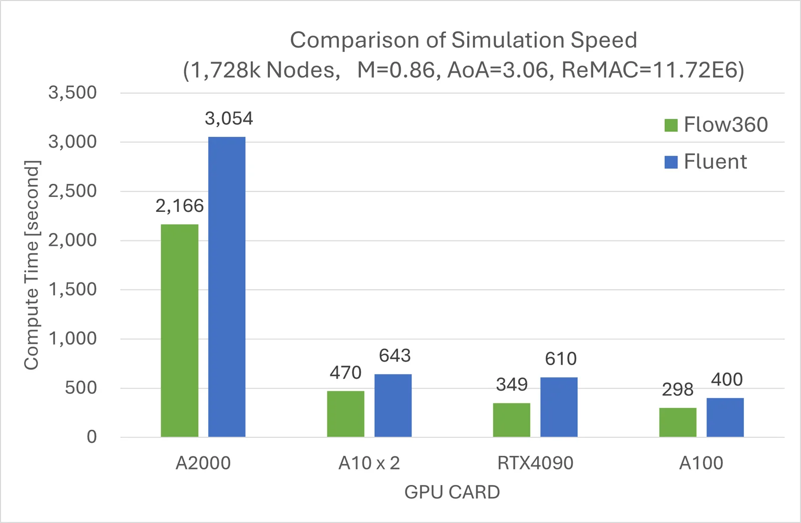
Commercial CFD codes are generally usable on up to 4 CPU cores with a base licence. On a legacy CPU code, 4 cores at this cell count take around 16 hours. That is a difference of roughly two orders of magnitude against the GPU runs.
| CPU | Runtime | CFD code | Cores |
|---|---|---|---|
| i9-10900X | 16.9 hours | Fluent DBNS | 4 |
| i9-10900X | 9.1 hours | Fluent DBNS | 10 |
4.2 Pressure distribution
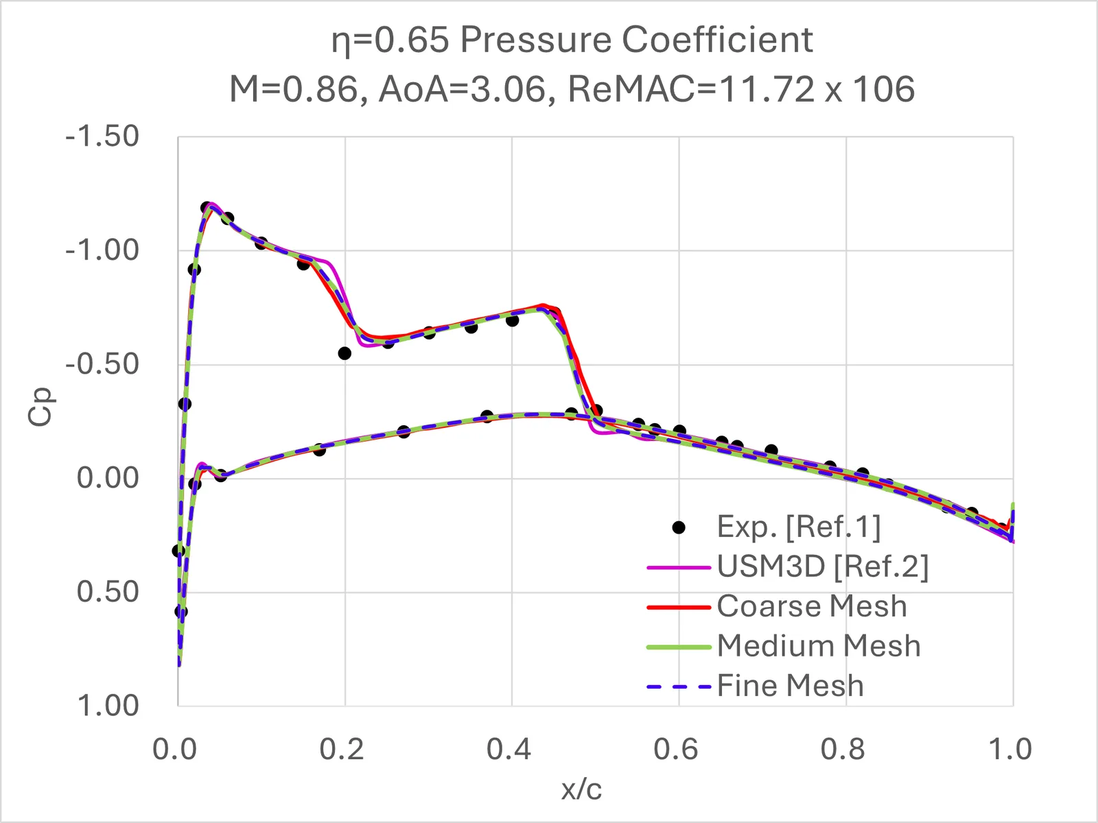
To examine how the results vary with cell count, pressure coefficients were extracted at each wing station and compared.
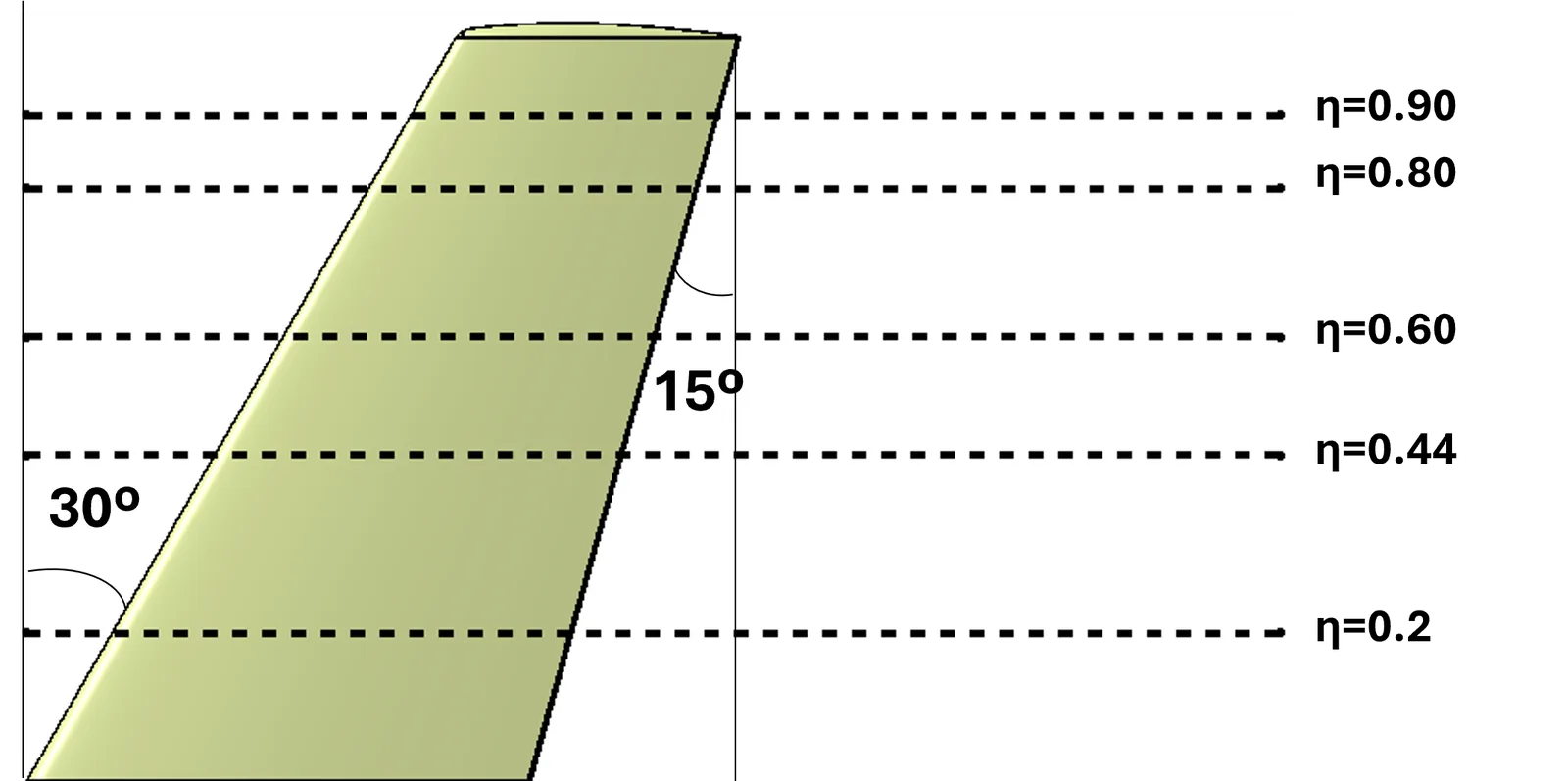
Overall the results agree well with the published experiments and with results in the literature, and the adverse pressure gradient produced by the shock is captured well. Towards the wing tip, at the 80% and 90% stations, the coarser mesh does show a small discrepancy in the adverse pressure gradient caused by the shocklet. The medium and fine meshes predict it well, which suggests the boundary-layer mesh on the coarse case is not dense enough.
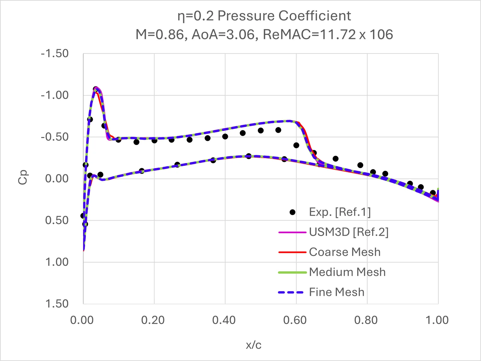
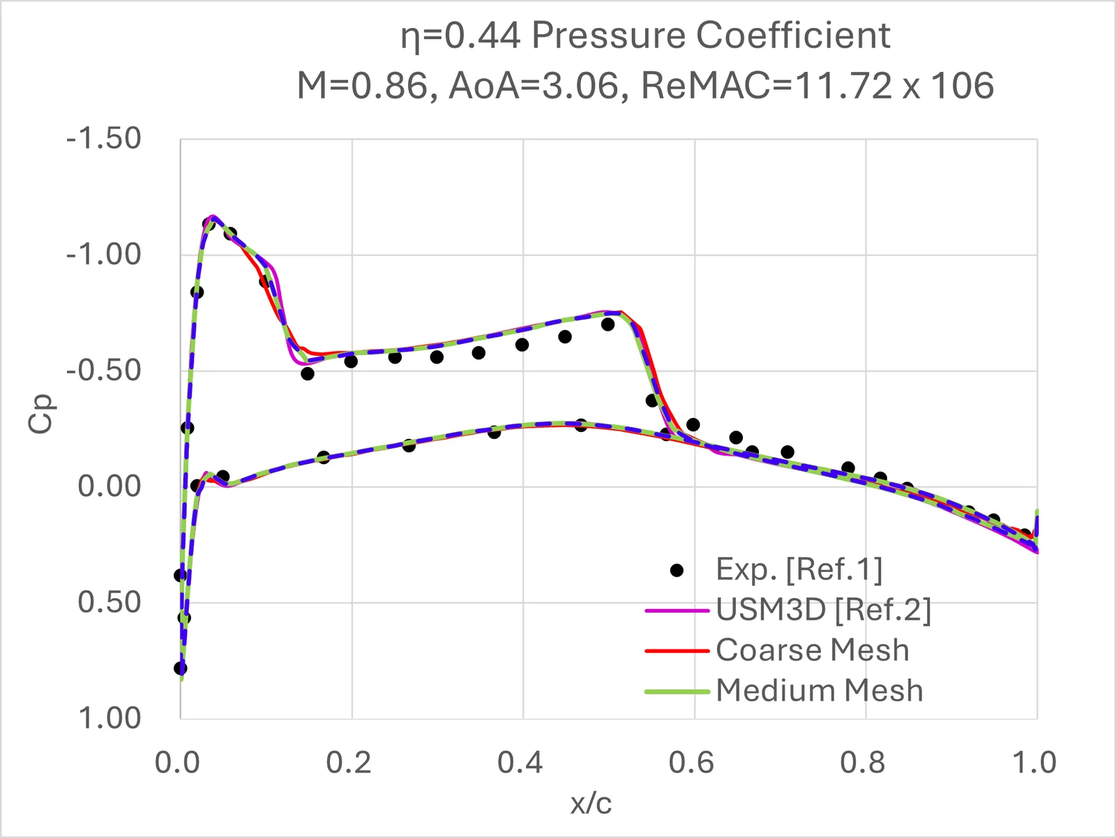
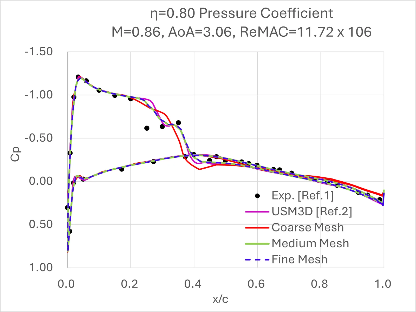
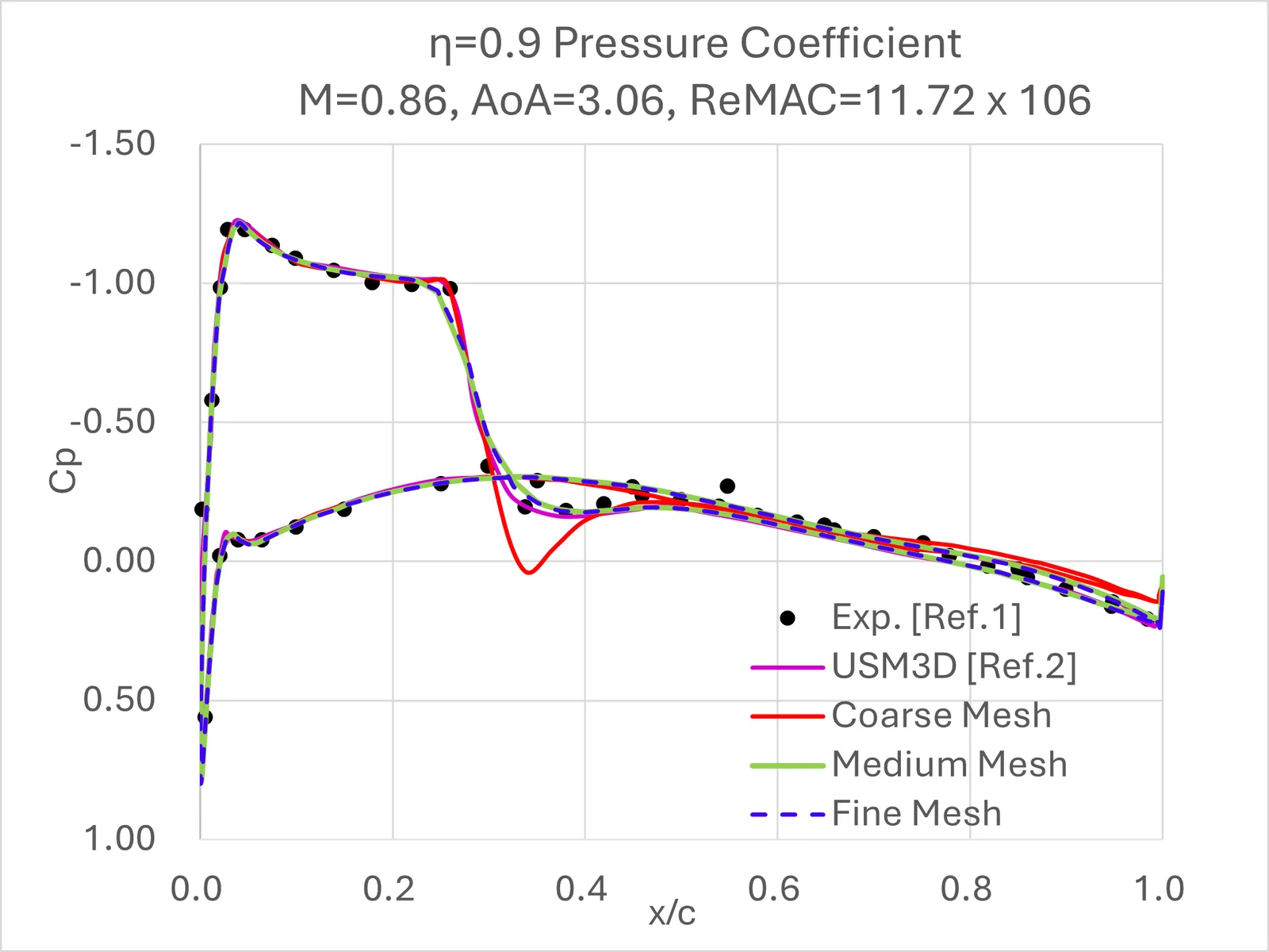
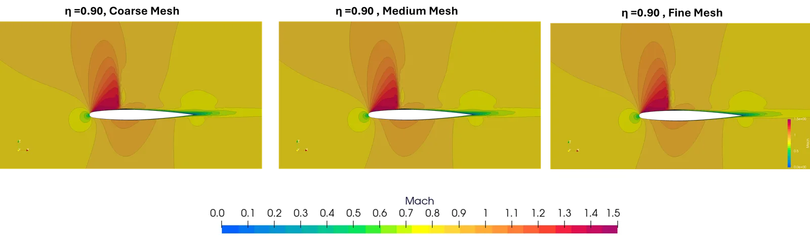
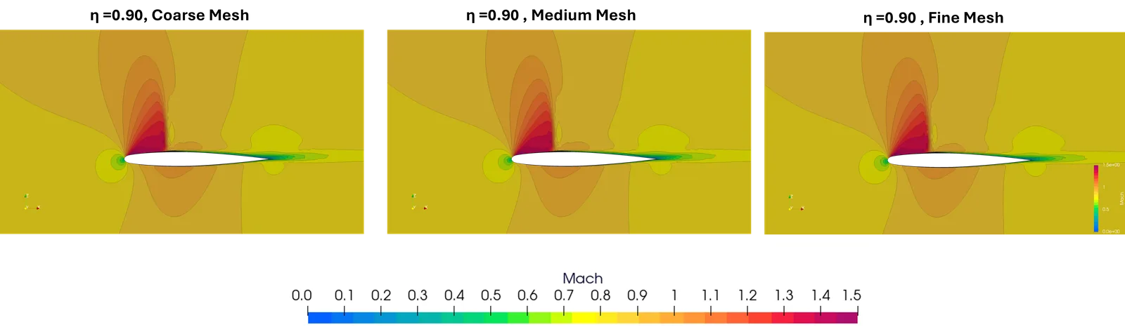
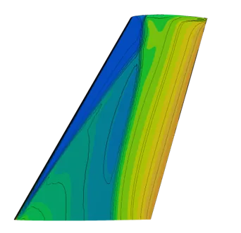
At the 80% and 90% stations the interaction between the boundary layer and the shock forms a shock shaped like the Greek letter lambda, λ. It develops along the freestream direction over the wing and produces the pressure pattern shown below on the suction surface. Capturing this phenomenon properly requires sufficient mesh resolution.
5. References
- Diskin, B., Anderson, W. K., Pandya, M. J., Rumsey, C. L., Thomas, J. L., Liu, Y., and Nishikawa, H., “Grid Convergence for Three-Dimensional Benchmark Turbulent Flows,” AIAA SciTech 2018 Forum, AIAA Paper 2018-1102, Jan. 2018. https://doi.org/10.2514/6.2018-1102
Want to know more about Flow360? Flow360 product page · Flexcompute documentation