1. The N1G model
CLEW works to provide fast, accurate CFD solutions for the aerospace and defence sector. This case study covers an analysis of the N1G supersonic missile test model.
The N1G is one of the models used to validate missile aerodynamics, because its wind-tunnel data is publicly available. The reference results were obtained in a supersonic wind tunnel. (See the references below for details.)
Flight conditions
- Mach number: 2.5
- Angle of attack: 6.05 degrees
- Altitude: 32,808.4 ft (10 km)
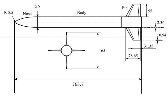
Principal dimensions
| Item | Dimension |
|---|---|
| Model length | 763.7 mm |
| Model diameter | 55 mm |
| Fin span | 165 mm |
| Model reference length | 2376 mm^2 |
2. Domain and mesh
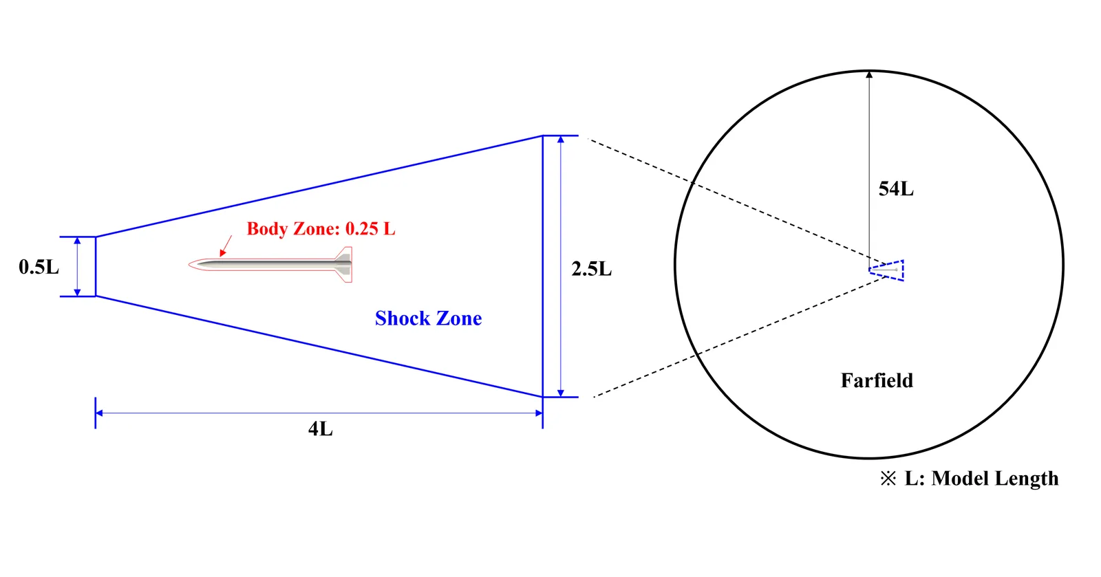
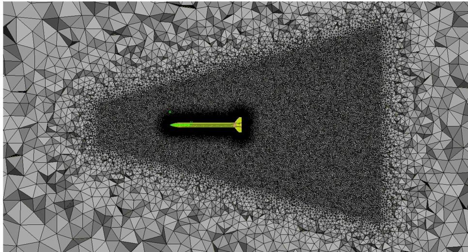
We built the hemispherical domain commonly used for external flow analysis. The region close to the model (body zone) was shaped to follow the N1G geometry so that the complex flow near the surface is captured. For the shock zone, a conical refinement region was defined so that the shocks around the vehicle in supersonic flight are resolved properly.
2.1 Surface mesh
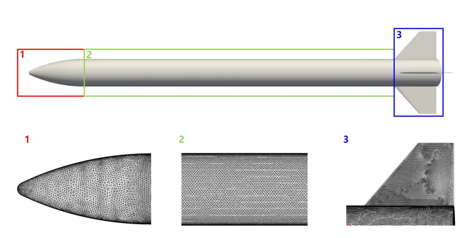
The surface mesh of the N1G model uses 144,781 triangles, configured as follows.
| Region | Element size (normalised by diameter) | Element size (absolute) |
|---|---|---|
| Missile body | 4.54 % | 2.5 mm |
| Fin | 1.81 % | 55 mm |
| Body offset refinement zone | 4.54 % | 2.5 mm |
| Cone refinement zone | 30.0 % | 16.5 mm |
| Number of surface elements | - | 144,781 |
2.2 Viscous layers
The boundary-layer mesh was configured as follows.
| Property | Value |
|---|---|
| First layer height | 0.036894 mm |
| Last ratio | 0.3 |
| Number of layers | 25 |
| Total layer height | 6.8876 mm |
2.3 Volume mesh
The volume mesh was generated with tetrahedra and exported as CGNS (or UGRID) for input to Flow360.
3. Solver setting
3.1 Flow conditions
Flow conditions were taken from Nenad et al., “Aerodynamic–structural missile fin optimization,” Aerospace Science and Technology, Vol. 65, 2017, pp. 26–45, so that the results can be compared directly.
- Freestream velocity: 745.825 [m/s]
- Temperature: 221.85 [K]
- Speed of sound: 298.33 [m/s]
- Density: 0.4048 [kg/m^3]
- Dynamic viscosity: 1.4565E-5 [N s/m2]
- Angle of attack: 6.05°
3.2 Navier–Stokes solver settings
In compressible flow, starting straight away with the solver at second order can make the run unstable, because a high-order scheme is applied before any flow field has been established. To avoid this, the analysis is split into two stages.
The first stage runs with the solver order set to first order. The second stage then continues with the order set to second order. For supersonic flow, limitVelocity and limitPressureDensity must both be set to true in the navierStokesSolver section of the case file.
fl.NavierStokesSolver(
    absolute_tolerance=1e-10,
    numerical_dissipation_factor=0.01,
    linear_solver=LinearSolver(max_iterations=50),
    low_mach_preconditioner=True,
    limit_velocity=True,
    limit_pressure_density=True,
)
4. Results
Mach contour
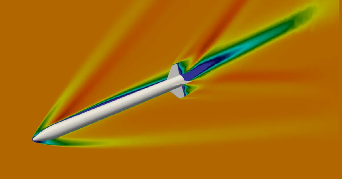
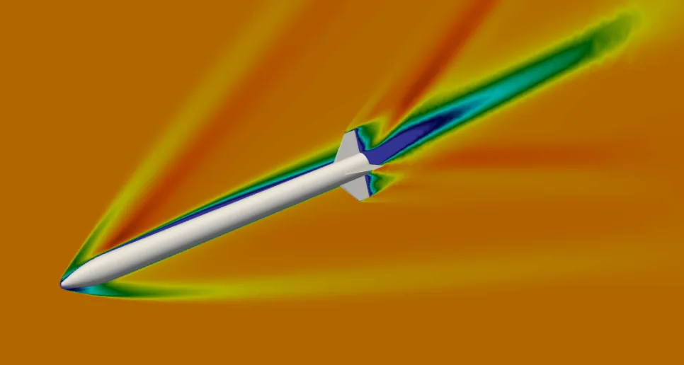
The Mach number field around the N1G is shown below. The visualisation confirms that the shocks at the nose cone and at the fins are reproduced properly.
Aerodynamic coefficient comparison
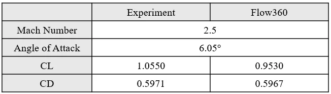
The table below compares the lift and drag coefficients predicted by Flow360 against the experiment. The experimental values are taken from the reference.
Want to know more about Flow360? Flow360 product page · Flexcompute documentation